Geophysical interpretation involves analyzing and integrating data obtained from various geophysical methods to infer the subsurface geology and its properties. This process is critical in many fields, including oil and gas exploration, mineral exploration, environmental studies, and engineering geology. The goal of geophysical interpretation is to create accurate subsurface models that can guide exploration, drilling, and other subsurface activities.

Objectives of Geophysical Interpretation

1. Subsurface Mapping:
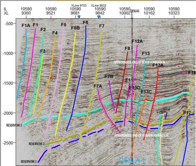
– Structural Interpretation: Identifying and mapping subsurface structures such as faults, folds, and stratigraphic boundaries.
– Lithological Interpretation: Differentiating between different rock types and their spatial distribution in the subsurface.

2. Resource Exploration:
– Hydrocarbon Reservoirs: Locating and characterizing potential oil and gas reservoirs.
– Mineral Deposits: Identifying and delineating mineral-rich zones.
– Groundwater Resources: Mapping aquifers and understanding their properties.

3. Environmental and Engineering Applications:
– Site Characterization: Assessing subsurface conditions for construction, waste disposal, and environmental remediation projects.
– Geohazard Assessment: Identifying and evaluating natural hazards such as landslides, subsidence, and seismic risks.

4. Reservoir Characterization:
– Porosity and Permeability: Estimating reservoir properties like porosity, permeability, and fluid saturation.
– Reservoir Geometry: Understanding the shape, size, and continuity of reservoirs.

Key Geophysical Methods Used in Interpretation

1. Seismic Methods:
– Seismic Reflection: The most widely used method, particularly in oil and gas exploration, it involves measuring the time it takes for seismic waves to travel through the Earth and reflect off subsurface layers. The resulting data is used to create images of the subsurface.
– Seismic Refraction: Used for mapping shallow subsurface structures, particularly in engineering and environmental studies.
– Seismic Attributes: Analysis of seismic data to extract additional information such as amplitude, frequency, and phase, which can provide insights into lithology, fluid content, and more.

2. Gravity and Magnetic Methods:
– Gravity Surveys: Measure variations in the Earth’s gravitational field caused by differences in rock density. These surveys are useful for identifying large-scale structures such as sedimentary basins, faults, and salt domes.
– Magnetic Surveys: Measure variations in the Earth’s magnetic field caused by the magnetic properties of subsurface rocks. These surveys are often used to map igneous and metamorphic rocks and can help in identifying mineral deposits.

3. Electrical and Electromagnetic Methods:
– Resistivity Surveys: Measure the resistance of the subsurface to electrical currents, which can be used to infer the presence of fluids, different rock types, and ore bodies.
– Electromagnetic (EM) Surveys: Measure the subsurface’s response to electromagnetic fields, useful for detecting conductive materials like ore bodies, groundwater, and contaminants.
– Induced Polarization (IP): Measures the ability of the subsurface to temporarily hold an electric charge, often used in mineral exploration.

4. Well Logging:
– Gamma Ray Logs: Measure natural radioactivity in rocks, useful for distinguishing between different types of sediments.
– Resistivity Logs: Provide information on the fluid content and porosity of rocks.
– Sonic Logs: Measure the speed of sound through rock formations, which can be related to rock density and porosity.
– Nuclear Magnetic Resonance (NMR) Logs: Provide direct measurements of porosity and pore size distribution.

5. Remote Sensing and Ground Penetrating Radar (GPR):
– Remote Sensing: Uses satellite or aerial imagery to detect surface features that may indicate underlying geological structures.
– GPR: A high-frequency electromagnetic method used to detect shallow subsurface features, particularly in environmental and engineering studies.

Process of Geophysical Interpretation

1. Data Acquisition:
– Survey Design: Careful planning of geophysical surveys, including the selection of appropriate methods, data coverage, and resolution, based on the objectives of the study.
– Data Collection: Acquisition of geophysical data through field surveys, drilling, or remote sensing.

2. Data Processing:
– Noise Reduction: Filtering and processing the raw data to remove noise and enhance the signal.
– Data Enhancement: Applying techniques such as migration (in seismic data) or inversion (in gravity and magnetic data) to improve the quality of the subsurface images.

3. Qualitative Interpretation:
– Structural Mapping: Identifying key structural features such as faults, folds, and stratigraphic boundaries from the processed data.
– Lithological Mapping: Inferring rock types and their distribution based on the geophysical signatures.

4. Quantitative Interpretation:
– Inversion Modeling: Converting geophysical data into physical property models (e.g., velocity, density, resistivity) that describe the subsurface.
– Reservoir Characterization: Estimating reservoir properties like porosity, permeability, and fluid saturation from geophysical data, often by integrating seismic data with well logs and other data sources.

5. Integration with Geological Data:
– Correlation with Well Logs: Comparing geophysical data with well log data to validate interpretations and refine subsurface models.
– Cross-Section Construction: Building cross-sections that integrate geological and geophysical data to provide a comprehensive view of the subsurface.
– 3D Modeling: Creating three-dimensional models that integrate all available data, allowing for more accurate predictions of subsurface features.

6. Uncertainty Analysis:
– Sensitivity Testing: Evaluating how variations in data or assumptions affect the interpretation.
– Risk Assessment: Identifying and quantifying the uncertainties in the geophysical interpretation, particularly in resource exploration.

Applications of Geophysical Interpretation

1. Oil and Gas Exploration:
– Prospect Identification: Locating potential hydrocarbon traps, such as anticlines, fault traps, and stratigraphic traps.
– Field Development: Guiding the placement of wells and infrastructure based on detailed subsurface models.
– Enhanced Oil Recovery (EOR): Monitoring reservoirs using time-lapse (4D) seismic data to optimize recovery techniques.

2. Mineral Exploration:
– Ore Body Delineation: Mapping the extent and geometry of ore bodies, particularly in complex geological settings.
– Exploration Targeting: Identifying new exploration targets based on geophysical anomalies.

3. Environmental and Engineering Studies:
– Contamination Assessment: Detecting and mapping subsurface contamination, such as leaks from storage tanks or landfills.
– Site Investigation: Characterizing subsurface conditions for construction projects, such as foundation stability or the presence of voids.

4. Groundwater Exploration:
– Aquifer Mapping: Locating and characterizing aquifers, including their depth, thickness, and quality.
– Saltwater Intrusion: Monitoring the extent of saltwater intrusion in coastal aquifers.

5. Geohazard Assessment:
– Landslide Mapping: Identifying and monitoring landslide-prone areas using geophysical techniques.
– Seismic Hazard Assessment: Evaluating fault activity and subsurface conditions that may contribute to earthquake risks.

Challenges in Geophysical Interpretation

1. Data Quality:
– Noise and Artifacts: Geophysical data often contain noise or artifacts that can obscure true geological signals, making interpretation challenging.
– Resolution Limits: The resolution of geophysical methods is often limited, particularly at great depths or in complex geological settings.

2. Ambiguity in Interpretation:
– Non-Uniqueness: Geophysical data can often be explained by multiple geological models, leading to ambiguity in interpretation.
– Complex Geology: In regions with complex geology, such as thrust belts or heavily faulted areas, interpreting geophysical data can be particularly challenging.

3. Integration Difficulties:
– Data Integration: Combining data from different geophysical methods, each with its own resolution and sensitivity, can be difficult and requires careful calibration.
– Scale Differences: Geophysical data often cover different spatial scales, making integration with geological data challenging.

4. Technological and Computational Challenges:
– Advanced Processing Needs: Modern geophysical interpretation often requires sophisticated processing techniques, such as 3D seismic inversion or machine learning, which can be computationally intensive.
– Software and Expertise: Interpreting geophysical data requires specialized software and expertise, which may not be readily available in all settings.

Conclusion

Geophysical interpretation is a critical process that enables geologists and geophysicists to understand the subsurface and make informed decisions in exploration, development, and environmental management. By integrating various geophysical methods with geological data, interpreters can create accurate subsurface models that guide exploration and development activities. Despite the challenges, advancements in technology and methodologies continue to improve the accuracy and reliability of geophysical interpretations, making it an indispensable tool in subsurface exploration.

Seismic attributes analysis is a powerful technique in geophysical interpretation that involves extracting and analyzing various quantitative measures from seismic data to enhance the understanding of subsurface features. These attributes can provide insights into geological structures, stratigraphy, and reservoir properties, often revealing details that are not easily discernible from conventional seismic data alone.

Objectives of Seismic Attributes Analysis

1. Enhanced Interpretation of Subsurface Features:
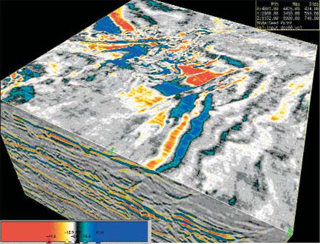
– Structural Analysis: Detecting and visualizing faults, fractures, folds, and other structural features.
– Stratigraphic Interpretation: Identifying and mapping depositional environments, unconformities, and stratigraphic sequences.
– Reservoir Characterization: Estimating reservoir properties such as porosity, permeability, lithology, and fluid content.

2. Improvement of Seismic Resolution:
– Detail Enhancement: Enhancing the visibility of subtle features, such as thin beds or small-scale structures, that may not be apparent in conventional seismic data.
– Noise Reduction: Isolating meaningful geological signals from seismic noise.

3. Risk Reduction in Exploration and Development:
– Prospect Identification: Identifying potential hydrocarbon traps and sweet spots within reservoirs.
– Well Placement Optimization: Guiding the positioning of exploration and production wells to maximize success rates and optimize recovery.

Types of Seismic Attributes

Seismic attributes can be broadly categorized into different types based on the kind of information they provide:

1. Amplitude Attributes:
– Root Mean Square (RMS) Amplitude: Measures the energy of the seismic signal, often used to identify bright spots, which may indicate the presence of hydrocarbons.
– Instantaneous Amplitude (Envelope): Represents the instantaneous energy of the seismic trace, highlighting amplitude anomalies that may correspond to geological features.
– Reflection Strength: Similar to RMS amplitude, used to indicate changes in lithology or fluid content.

2. Phase Attributes:
– Instantaneous Phase: Measures the phase angle of the seismic wave at each point in time, useful for identifying continuity of reflectors and distinguishing between constructive and destructive interference.
– Phase Rotation: Helps in phase correction and aligning seismic data for better interpretation of stratigraphic features.

3. Frequency Attributes:
– Instantaneous Frequency: Represents the dominant frequency of the seismic signal at each point in time, which can help in identifying variations in layer thickness, fluid content, and lithology.
– Dominant Frequency: The frequency at which the seismic energy is concentrated, often used to infer changes in sedimentary facies or reservoir characteristics.
– Spectral Decomposition: Decomposes seismic data into its frequency components to analyze thin beds, stratigraphic details, and subtle changes in reservoir properties.

4. Geometric Attributes:
– Dip and Azimuth: Measures the orientation of seismic reflectors, which helps in identifying structural features like faults, folds, and stratigraphic boundaries.
– Coherence (Similarity): Measures the similarity between adjacent seismic traces, highlighting discontinuities such as faults, channels, and pinch-outs.
– Curvature: Quantifies the bending of seismic reflectors, useful for identifying fold structures, fractures, and fault-related deformation.
– Edge Detection (e.g., Sobel filter): Enhances the visibility of edges and boundaries in the seismic data, often used to delineate faults, channels, and stratigraphic features.

5. Avo (Amplitude Versus Offset) Attributes:
– Intercept and Gradient: Analyzes the change in amplitude with offset (distance between source and receiver), which can indicate the presence of hydrocarbons, gas, or fluid contacts.
– AVO Classifications: Categorizes reservoirs based on their AVO response, helping to distinguish between gas, oil, and water zones.

6. Advanced Attributes:
– Seismic Inversion: Converts seismic reflection data into acoustic impedance or other rock properties, providing more direct information about lithology and fluid content.
– Elastic Impedance: A generalized form of acoustic impedance that incorporates information from AVO analysis, used to differentiate between different lithologies and fluid types.
– Texture and Attribute Combinations: Combines multiple attributes using machine learning or statistical methods to enhance interpretation and detect complex geological features.

Workflow for Seismic Attributes Analysis

1. Data Preparation:
– Seismic Data Conditioning: Applying preprocessing steps such as noise reduction, deconvolution, and migration to improve data quality before attribute extraction.
– Attribute Selection: Choosing the appropriate attributes based on the geological objectives, such as fault detection, reservoir characterization, or stratigraphic analysis.

2. Attribute Calculation:
– Single-Trace Attributes: Calculating attributes from individual seismic traces, such as amplitude, phase, or frequency attributes.
– Multi-Trace Attributes: Calculating attributes that involve multiple traces, such as coherence or curvature, which require spatial analysis of the data.

3. Attribute Visualization:
– Time Slices and Horizon Slices: Visualizing attributes along selected horizons or time slices to highlight geological features.
– Cross-Plotting: Plotting one attribute against another to identify trends and relationships between different properties, such as amplitude versus frequency or impedance versus porosity.

4. Interpretation and Integration:
– Geological Interpretation: Linking seismic attributes to geological features, such as faults, fractures, channels, and stratigraphic sequences.
– Integration with Other Data: Combining seismic attributes with well logs, core data, and other geological or geophysical information to refine the subsurface model.

5. Validation and Calibration:
– Correlation with Well Data: Comparing seismic attributes with well data to validate interpretations and calibrate attribute responses to known lithologies or fluid types.
– Sensitivity Analysis: Evaluating the robustness of attribute interpretation by testing different parameters, data conditioning techniques, or attribute combinations.

6. Advanced Analysis and Machine Learning:
– Pattern Recognition: Using pattern recognition techniques to identify geological features within seismic attributes, such as channels, reefs, or fracture networks.
– Machine Learning: Applying machine learning algorithms to classify seismic attributes, predict reservoir properties, or automate the identification of geological features.

Applications of Seismic Attributes Analysis

1. Fault and Fracture Detection:
– Fault Imaging: Enhancing the visibility of faults and fractures using attributes like coherence, curvature, and edge detection.
– Fracture Characterization: Understanding fracture density, orientation, and connectivity, which are crucial for reservoir quality in fractured reservoirs.

2. Stratigraphic Interpretation:
– Channel and Reef Identification: Detecting and mapping channels, reefs, and other stratigraphic features using amplitude, frequency, and geometric attributes.
– Sequence Stratigraphy: Analyzing stratigraphic sequences, unconformities, and depositional environments to build a sequence stratigraphic framework.

3. Reservoir Characterization:
– Lithology and Fluid Prediction: Estimating lithology, porosity, and fluid content using attributes like seismic inversion, AVO, and impedance.
– Sweet Spot Identification: Identifying high-quality reservoir zones with favorable properties, such as high porosity or hydrocarbon saturation.

4. Hydrocarbon Exploration:

• Direct Hydrocarbon Indicators (DHIs): Identifying bright spots, flat spots, and other seismic anomalies that may indicate the presence of hydrocarbons.
  – Prospect De-Risking: Reducing exploration risk by using seismic attributes to better understand the subsurface before drilling.

5. Time-Lapse (4D) Seismic Monitoring:
– Reservoir Monitoring: Tracking changes in reservoir properties over time using seismic attributes, particularly during production or enhanced oil recovery (EOR) operations.
– Production Optimization: Adjusting production strategies based on the interpretation of time-lapse seismic data.

Challenges in Seismic Attributes Analysis

1. Attribute Selection and Interpretation:
– Non-Uniqueness: Different geological features can produce similar seismic attribute responses, leading to ambiguous interpretations.
– Attribute Overload: With the availability of many attributes, selecting the most relevant ones for a particular interpretation task can be challenging.

2. Data Quality and Resolution:
– Noise and Artifacts: Poor data quality or artifacts in the seismic data can lead to misleading attribute responses.
– Resolution Limits: The resolution of seismic data, particularly in deep or complex areas, may limit the effectiveness of certain attributes.

3. Integration with Other Data:
– Data Integration: Combining seismic attributes with other geophysical, geological, and well data requires careful calibration and validation.
– Scale Differences: Attributes derived from seismic data may need to be reconciled with higher-resolution well log or core data, which can differ in scale.

4. Computational Complexity:
– Advanced Processing Requirements: Calculating and interpreting some seismic attributes, especially those involving machine learning or 3D analysis, can be computationally intensive.
– Software and Expertise: Specialized software and expertise are required to fully leverage the potential of seismic attributes.

Conclusion

Seismic attributes analysis is a versatile and powerful tool that enhances the interpretation of seismic data, enabling geophysicists and geologists to gain deeper insights into the subsurface. By extracting and analyzing various attributes, interpreters can better understand structural, stratigraphic, and reservoir characteristics, leading to more informed decisions in exploration, development, and production. Despite the challenges, advancements in technology, data processing, and interpretation techniques continue to expand the applications and accuracy of seismic attributes analysis, making it an essential component of modern geophysical interpretation.

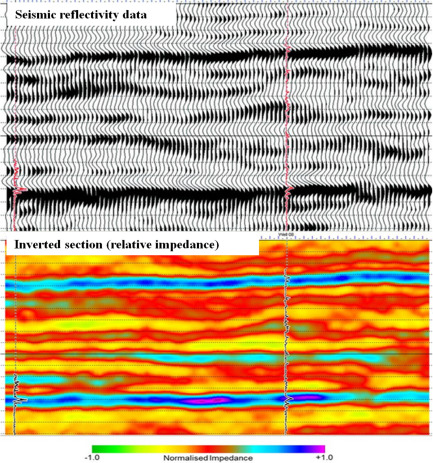
Seismic inversion is a geophysical technique used to convert seismic reflection data into a quantitative rock property model of the subsurface, such as acoustic impedance, shear impedance, or other elastic properties. This process is essential in reservoir characterization, as it provides more detailed and accurate information about the subsurface than raw seismic data alone. Seismic inversion helps in interpreting the lithology, porosity, fluid content, and other important reservoir characteristics.

Objectives of Seismic Inversion

1. Quantitative Interpretation:
– Rock Property Estimation: Converting seismic reflection data into rock properties like acoustic impedance, density, and shear impedance, which are directly related to lithology, porosity, and fluid content.
– Reservoir Characterization: Enhancing the understanding of reservoir properties, including the distribution of hydrocarbons, porosity, and fluid saturation.

2. Improvement of Subsurface Imaging:
– Resolution Enhancement: Providing higher-resolution images of the subsurface, which helps in identifying thin beds and subtle geological features.
– Noise Reduction: Filtering out noise and improving the signal-to-noise ratio to produce more accurate and interpretable subsurface models.

3. Risk Reduction in Exploration and Development:
– De-Risking Prospects: Reducing exploration risk by providing more reliable information about the subsurface, which helps in making informed drilling decisions.
– Optimization of Well Placement: Guiding the placement of wells based on detailed rock property models, thereby improving recovery and reducing costs.

Types of Seismic Inversion

1. Deterministic Inversion:

– Post-Stack Inversion: A common and straightforward approach where seismic data after stacking (post-stack) are inverted to produce acoustic impedance models. It typically provides a smooth and band-limited representation of the subsurface.
– Pre-Stack Inversion: Involves inverting seismic data before stacking (pre-stack) to obtain elastic properties such as P-wave impedance, S-wave impedance, and density. Pre-stack inversion can provide more detailed information about lithology and fluid content.

2. Geostatistical Inversion:
– Stochastic Inversion: Incorporates both seismic data and well log information to produce multiple realizations of the subsurface model, accounting for uncertainty. This method is useful for reservoir characterization and risk assessment.
– Sequential Gaussian Simulation: A technique used in geostatistical inversion to generate realizations of rock properties by combining seismic data with spatial statistical models.

3. Simultaneous Inversion:
– Simultaneous AVO Inversion: Integrates amplitude variation with offset (AVO) information to simultaneously invert for multiple properties, such as P-wave and S-wave impedances, and density. This approach is particularly useful for distinguishing between lithology and fluid effects.
– Simultaneous Inversion of Multiple Seismic Data Sets: Combines different types of seismic data, such as P-wave and S-wave data, to create a more comprehensive model of the subsurface.

4. Model-Based Inversion:
– Layer-Based Inversion: Uses a priori geological models and well log data to guide the inversion process, producing models that are consistent with known geology.
– Bayesian Inversion: Applies Bayesian statistics to incorporate prior information and uncertainty into the inversion process, producing probabilistic models of the subsurface.

Workflow for Seismic Inversion

1. Data Preparation:
– Seismic Data Conditioning: Preprocessing of seismic data to remove noise, multiple reflections, and other artifacts. This step is crucial for ensuring the quality of the inversion results.
– Well Log Calibration: Using well log data to calibrate the seismic inversion process. This involves correlating seismic data with well logs to create a reliable starting model.

2. Initial Model Building:
– Low-Frequency Model: Constructing a low-frequency model that captures the broad trends in the subsurface, usually derived from well log data and geological knowledge. This model is combined with the seismic data to guide the inversion process.
– Initial Guess Model: Creating an initial guess of the subsurface properties, which serves as a starting point for the inversion algorithm.

3. Inversion Process:
– Inversion Algorithm Selection: Choosing the appropriate inversion method (e.g., deterministic, stochastic, pre-stack) based on the objectives and available data.
– Iteration and Optimization: Iteratively adjusting the model to minimize the difference between the synthetic seismic data (generated from the model) and the observed seismic data. This process is guided by optimization techniques.

4. Model Validation:
– Comparison with Well Data: Validating the inversion results by comparing the inverted model with well log data. This step ensures that the model is consistent with known subsurface information.
– Residual Analysis: Analyzing the differences between the observed and synthetic seismic data to assess the quality of the inversion and identify any discrepancies.

5. Interpretation and Integration:
– Rock Property Interpretation: Interpreting the inverted rock property models to gain insights into lithology, fluid content, and other reservoir characteristics.
– Integration with Geological Models: Combining the seismic inversion results with geological models, well logs, and other geophysical data to create a comprehensive subsurface model.

6. Uncertainty Analysis:
– Sensitivity Testing: Assessing the sensitivity of the inversion results to different parameters, such as the initial model, seismic data quality, and inversion settings.
– Probabilistic Inversion: Generating multiple realizations of the subsurface model to quantify uncertainty and assess the risk associated with different interpretations.

Applications of Seismic Inversion

1. Reservoir Characterization:
– Lithology Discrimination: Distinguishing between different rock types, such as sandstones, shales, and carbonates, based on their seismic response.
– Fluid Identification: Identifying the presence and distribution of fluids, such as oil, gas, and water, within the reservoir.
– Porosity Estimation: Estimating porosity distribution within the reservoir, which is critical for understanding reservoir quality and potential recovery.

2. Stratigraphic Interpretation:
– Sequence Stratigraphy: Analyzing stratigraphic sequences and identifying key boundaries, such as unconformities and flooding surfaces.
– Thin Bed Analysis: Detecting and characterizing thin beds that may be below the resolution of conventional seismic data but can be resolved through inversion.

3. Hydrocarbon Exploration:
– Prospect Identification: Identifying potential hydrocarbon-bearing zones based on anomalies in rock properties derived from seismic inversion.
– Direct Hydrocarbon Indicators (DHIs): Detecting seismic attributes or inversion results that may indicate the presence of hydrocarbons, such as low acoustic impedance anomalies.

4. Enhanced Oil Recovery (EOR):
– Reservoir Monitoring: Using time-lapse (4D) seismic inversion to monitor changes in reservoir properties during production and EOR operations.
– Production Optimization: Adjusting production strategies based on the evolving understanding of the reservoir provided by seismic inversion.

5. Geomechanical Modeling:
– Stress Field Analysis: Estimating rock mechanical properties, such as Young’s modulus and Poisson’s ratio, which are essential for understanding the stress field and predicting geomechanical behavior.
– Fracture Prediction: Identifying zones of potential fracturing or fault reactivation based on seismic inversion results.

Challenges in Seismic Inversion

1. Data Quality and Resolution:
– Seismic Noise: Noise in the seismic data can lead to inaccuracies in the inversion results. High-quality, noise-free data are essential for reliable inversion.
– Frequency Content: Seismic data are typically band-limited, meaning they do not contain the full range of frequencies needed to resolve all subsurface details. The low-frequency model helps address this, but it can introduce bias.

2. Non-Uniqueness of Solutions:
– Multiple Models: Seismic inversion is inherently non-unique, meaning that different models can produce similar seismic responses. This can lead to ambiguity in interpretation.
– Model Dependence: The inversion results are often dependent on the initial model, which can bias the outcome if not carefully constructed.

3. Computational Complexity:
– High Computational Costs: Seismic inversion, especially pre-stack and stochastic methods, can be computationally intensive, requiring significant processing power and time.
– Advanced Software Requirements: Specialized software and expertise are needed to perform seismic inversion effectively, which may not be readily available in all settings.

4. Integration with Other Data:
– Data Integration Challenges: Combining seismic inversion results with well logs, geological models, and other geophysical data can be challenging due to differences in scale, resolution, and data quality.
– Calibration and Validation: Ensuring that the inversion results are consistent with well log data and other ground truth information is crucial for reliable interpretation.

Conclusion

Seismic inversion is a critical tool in geophysical exploration and reservoir characterization, providing detailed and quantitative models of the subsurface that are essential for informed decision-making. By converting seismic data into rock properties, seismic inversion helps geoscientists and engineers better understand the distribution of lithology, porosity, and fluids in the subsurface. Despite challenges such as non-uniqueness, data quality issues, and computational complexity, advances in inversion techniques and software continue to improve the accuracy and applicability of seismic inversion, making it an indispensable part of modern geophysical interpretation.

AVO (Amplitude Versus Offset) rock physics is a crucial aspect of geophysics that focuses on understanding how seismic wave amplitudes change with increasing distance (offset) from the seismic source to the receiver and how these changes relate to the physical properties of rocks, such as porosity, lithology, fluid content, and pressure. AVO analysis helps geoscientists and reservoir engineers interpret seismic data to better characterize subsurface formations, particularly in identifying hydrocarbon reservoirs and understanding fluid distributions.

Fundamentals of AVO and Rock Physics

1. Seismic Wave Propagation:
– Reflection Coefficients: When a seismic wave encounters an interface between two different rock layers, part of the wave is reflected back to the surface, and part of it continues to propagate. The amplitude of the reflected wave is determined by the contrast in acoustic impedance (product of rock density and seismic velocity) between the two layers.
– Offset Dependence: The angle of incidence (related to offset) affects the reflection coefficient, and therefore the amplitude of the reflected wave. AVO analysis examines how these amplitudes vary with offset to infer rock and fluid properties.

2. Rock Properties and Seismic Response:
– Acoustic Impedance: A primary rock property influencing seismic reflection. It is dependent on both the density of the rock and the velocity of seismic waves through it. Variations in acoustic impedance across layers result in different reflection amplitudes.
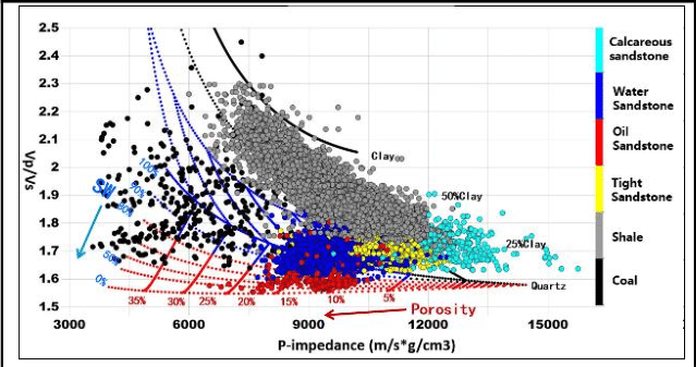
– Shear and Compressional Velocities: Compressional (P-wave) and shear (S-wave) velocities are sensitive to rock type, porosity, and fluid saturation. The ratio of these velocities (Vp/Vs) is a key indicator in AVO analysis, as different fluids (gas, oil, water) and lithologies yield distinct Vp/Vs ratios.
– Elastic Moduli: Rock elasticity, represented by moduli such as bulk modulus, shear modulus, and Young’s modulus, also affects seismic wave propagation and can be related to rock properties through rock physics models.

3. Fluid and Lithology Effects:
– Gassmann’s Equations: These are used to predict the effect of fluid substitution on seismic velocities in a porous rock. By applying these equations, one can model how the presence of different fluids (e.g., water, oil, gas) will influence the seismic response.
– Porosity and Saturation: Higher porosity generally decreases seismic velocities and acoustic impedance, while fluid saturation can significantly alter the AVO response. Gas, in particular, causes a marked reduction in P-wave velocity, leading to a strong AVO anomaly.

AVO Analysis and Interpretation

1. AVO Classification:
– Class I: High impedance contrast, typically characterized by decreasing amplitude with offset. Often associated with brine-saturated sandstones.
– Class II: Small or zero impedance contrast, showing little change in amplitude with offset. Common in low-contrast interfaces, such as between similar lithologies.
– Class III: Low impedance contrast, with increasing amplitude with offset. Often indicative of gas sands.
– Class IV: Very low impedance contrast, with a polarity reversal at near offsets and increasing amplitude at far offsets. Also associated with gas sands but with different rock properties compared to Class III.

2. AVO Crossplotting:
– Intercept vs. Gradient Plot: A common technique where the intercept (amplitude at zero offset) is plotted against the gradient (rate of change of amplitude with offset). This helps distinguish between different AVO classes and can indicate the presence of hydrocarbons.
– Fluid and Lithology Discrimination: By analyzing the position of data points on an AVO crossplot, geoscientists can infer the type of fluid present and the lithology of the reservoir rock.

3. AVO Inversion:
– Elastic Impedance Inversion: Extending AVO analysis to invert seismic data for elastic properties such as P-wave impedance, S-wave impedance, and density. This process helps in constructing a detailed subsurface model that can predict reservoir properties.
– Simultaneous Inversion: Integrates AVO data from multiple offsets to simultaneously invert for multiple rock properties, improving the accuracy of lithology and fluid predictions.

Applications of AVO Rock Physics

1. Hydrocarbon Exploration:
– Direct Hydrocarbon Indicators (DHIs): AVO anomalies can act as DHIs, signaling the presence of hydrocarbons. Class III and Class IV AVO responses are particularly useful in identifying gas reservoirs.
– Prospect Risking: AVO analysis helps reduce exploration risk by providing additional evidence for the presence of hydrocarbons, aiding in the decision-making process for drilling.

2. Reservoir Characterization:
– Fluid Saturation Estimation: By combining AVO analysis with rock physics models, geoscientists can estimate the fluid saturation in the reservoir, helping to distinguish between oil, gas, and water.
– Porosity and Lithology Mapping: AVO analysis provides insights into the porosity distribution and lithological variations within the reservoir, which are crucial for reservoir modeling and simulation.

3. Enhanced Oil Recovery (EOR):
– Monitoring Fluid Movement: Time-lapse (4D) AVO analysis can monitor changes in fluid distribution during EOR operations, such as waterflooding or CO2 injection, helping to optimize recovery strategies.

4. Geomechanical Applications:
– Stress and Fracture Analysis: AVO analysis can be used to study changes in the stress field or to identify fractured zones, which are important for wellbore stability and fracture stimulation planning.

Challenges in AVO Rock Physics

1. Data Quality:
– Noise and Multiples: Seismic data must be of high quality, with minimal noise and multiples, to obtain reliable AVO results. Poor data quality can lead to misinterpretation of AVO anomalies.
– Offset Coverage: Adequate offset coverage is essential for accurate AVO analysis. Limited offsets may not fully capture the amplitude variation, leading to incomplete or biased interpretations.

2. Non-uniqueness:
– Ambiguity in Interpretation: AVO responses can be influenced by multiple factors, such as changes in lithology, fluid content, and pore pressure. This non-uniqueness can make it challenging to isolate the exact cause of an AVO anomaly.
– Complex Subsurface Conditions: Heterogeneous subsurface conditions, such as variable lithologies or anisotropy, can complicate AVO analysis and require advanced modeling techniques to interpret correctly.

3. Rock Physics Modeling:
– Assumptions and Approximations: Rock physics models used in AVO analysis rely on assumptions that may not always hold true in complex geological settings. For example, Gassmann’s equations assume isotropy and homogeneity, which may not be accurate in fractured or anisotropic formations.
– Calibration with Well Data: Accurate AVO interpretation requires calibration with well log data. Discrepancies between seismic and well data can lead to incorrect conclusions if not properly accounted for.

Conclusion

AVO rock physics plays a pivotal role in modern geophysical exploration and reservoir characterization. By analyzing how seismic amplitudes vary with offset, AVO analysis provides valuable insights into the subsurface, particularly in identifying hydrocarbons and understanding reservoir properties. Despite the challenges of data quality, non-uniqueness, and complex subsurface conditions, advances in AVO techniques and rock physics modeling continue to enhance the accuracy and reliability of this method, making it an essential tool for geoscientists and engineers in the energy industry.

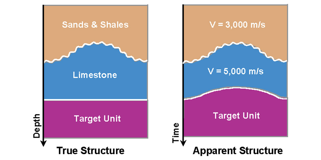
Depth conversion is a crucial process in geophysics and subsurface exploration, involving the transformation of seismic reflection data from the time domain to the depth domain. This process is essential because seismic data are initially recorded in terms of two-way travel time (the time it takes for a seismic wave to travel from the surface to a reflector and back), but for practical purposes such as drilling and reservoir modeling, it is necessary to understand the actual depth of subsurface structures.

Importance of Depth Conversion

1. Accurate Subsurface Mapping:
– Depth conversion allows geoscientists to create accurate depth maps of subsurface geological structures, which are critical for identifying potential hydrocarbon reservoirs, aquifers, and other resources.
– It provides a more precise location of geological features such as faults, folds, and stratigraphic traps.

2. Well Planning and Drilling:
– Depth conversion is essential for well planning, as it determines the true depth at which drilling should occur to reach the target reservoir.
– It helps in avoiding drilling hazards by accurately predicting the depth of potential overpressured zones or other geological risks.

3. Reservoir Characterization:
– In-depth domain data, geoscientists can better characterize reservoirs, including their geometry, thickness, and volume.
– This process aids in the estimation of reserves and enhances the accuracy of reservoir models used in production planning.

4. Integration with Other Data:
– Depth conversion allows the integration of seismic data with well logs, core data, and other geological information, creating a coherent subsurface model.
– It enables more accurate geological and geophysical interpretations by correlating time-domain seismic data with actual depth measurements.

Methods of Depth Conversion

1. Vertical Depth Conversion:
– Constant Velocity Method: A simple method where a constant average velocity is used to convert time to depth. It is often used in initial stages or in areas with uniform velocity structures.
– Layer Cake Model: This method assumes that the subsurface is made up of horizontal layers, each with a constant velocity. The time-depth conversion is performed layer by layer, using the velocity for each layer.
– Time-Depth Curve: Derived from well data, these curves represent the relationship between time and depth at specific well locations. They are often used to guide depth conversion in nearby areas.

2. Seismic Velocity Modeling:
– Velocity Analysis: Involves determining seismic velocities at various depths and offsets from seismic data. This can be done using techniques such as semblance analysis, stacking velocity analysis, or tomography.
– Interval Velocity Method: Seismic interval velocities are derived from stacking velocities or well data and used to convert time to depth. The interval velocity is the average velocity between two depth points.
– RMS Velocity: Root Mean Square (RMS) velocity is another common method used in depth conversion, which averages the squared velocities over a depth interval.

3. Geostatistical Methods:
– Kriging and Cokriging: Geostatistical methods like kriging are used to interpolate velocity fields or depth surfaces. These methods take into account spatial variability and uncertainty, providing a more accurate depth conversion.
– Stochastic Modeling: Incorporates the randomness and uncertainty in velocity models by using multiple realizations of velocity fields to assess the range of possible depth conversions.

4. Depth Migration:
– Pre-stack Depth Migration (PSDM): An advanced technique that directly migrates seismic data from the time domain to the depth domain, taking into account complex velocity variations. PSDM is particularly useful in areas with complex geology, such as salt bodies or steeply dipping beds.
– Post-stack Depth Migration: Applied after stacking the seismic data, this method converts time-migrated seismic data into depth. It is less accurate than PSDM but computationally simpler and faster.

5. Hybrid Approaches:
– Layer-based and Gridded Velocity Models: Combining both layer-based approaches and gridded velocity models allows for more detailed and accurate depth conversion, particularly in areas with varying velocity structures.
– Integrated Well-Seismic Calibration: Using well data to calibrate seismic velocities improves the accuracy of depth conversion, particularly in heterogeneous reservoirs.

Challenges in Depth Conversion

1. Velocity Model Accuracy:
– Complex Geology: In areas with complex geology, such as folded or faulted regions, creating an accurate velocity model is challenging, leading to uncertainties in depth conversion.
– Velocity Anisotropy: The assumption of isotropic velocities (same velocity in all directions) can lead to errors in depth conversion, especially in areas with anisotropic conditions, such as shales.

2. Data Quality and Availability:
– Sparse Well Data: Limited well control can result in inaccurate time-depth relationships, affecting the reliability of the depth conversion.
– Seismic Data Resolution: Low-resolution seismic data can lead to poor velocity estimation and depth conversion, particularly in deeper sections or complex geological settings.

3. Uncertainty and Ambiguity:
– Multiple Interpretations: Different velocity models can produce varying depth conversion results, leading to uncertainty in the final depth maps.
– Non-uniqueness: Multiple combinations of velocity and time can result in the same depth, making it difficult to choose the correct model.

4. Integration with Other Data:
– Consistency with Well Data: Ensuring that depth-converted seismic data is consistent with well data can be challenging, particularly when there are discrepancies between seismic velocities and well log measurements.
– Cross-disciplinary Challenges: Integrating depth conversion with geological and reservoir engineering models requires cross-disciplinary expertise and careful consideration of different data types and scales.

Applications of Depth Conversion

1. Exploration and Prospect Evaluation:
– Depth conversion helps in accurately mapping prospects and evaluating their potential for hydrocarbon accumulation.
– It aids in the identification of structural and stratigraphic traps and in assessing the size and depth of potential reservoirs.

2. Reservoir Management:
– Accurate depth maps are essential for reservoir management, including well placement, reservoir modeling, and production optimization.
– Depth conversion provides critical input for volumetric calculations, reserve estimation, and reservoir simulation models.

3. Geohazard Assessment:
– Depth conversion is used to identify and assess geohazards, such as overpressured zones, fault zones, and salt bodies, which can pose risks during drilling.
– It helps in planning safe drilling operations and avoiding hazardous areas.

4. Enhanced Oil Recovery (EOR):
– In EOR projects, depth conversion is used to monitor the movement of injected fluids and to optimize the placement of injection and production wells.
– It assists in tracking changes in reservoir conditions over time and in updating reservoir models.

Conclusion

Depth conversion is a fundamental process in geophysical exploration and reservoir characterization, transforming seismic data from the time domain to the depth domain. By creating accurate depth maps of subsurface structures, depth conversion aids in well planning, reservoir management, and risk assessment. Despite challenges related to velocity model accuracy, data quality, and uncertainty, advances in seismic velocity modeling, depth migration, and geostatistical methods continue to enhance the reliability and accuracy of depth conversion, making it an indispensable tool in the oil and gas industry.

Seismic to well tie is a critical process in geophysics and petroleum exploration, involving the correlation of seismic data with well data to create a consistent and accurate interpretation of the subsurface. This process ensures that seismic reflections, typically recorded in time, are correctly aligned with the geological and petrophysical information obtained from well logs, which are measured in depth.

Importance of Seismic to Well Ties

1. Integration of Data:
– Aligning Time and Depth: Seismic to well ties align the seismic time domain data with the well depth domain data, allowing for accurate depth conversion and subsurface mapping.
– Consistent Interpretation: By correlating seismic data with well data, geoscientists can ensure that the geological interpretations derived from seismic data are consistent with the direct measurements from the well.

2. Improved Seismic Interpretation:
– Calibration of Seismic Data: The process helps calibrate seismic data, making it possible to accurately identify and map geological features such as faults, horizons, and reservoirs.
– Identification of Seismic Reflectors: Seismic to well ties assist in identifying the origin of specific seismic reflectors, helping to associate them with particular geological formations or lithological boundaries.

3. Reservoir Characterization:
– Accurate Reservoir Mapping: Tying seismic data to well logs allows for more accurate delineation of reservoir boundaries, thickness, and heterogeneity.
– Enhanced Reservoir Models: The process provides critical input for building detailed and accurate reservoir models, which are essential for reserve estimation and production planning.

4. Well Planning and Drilling:
– Target Identification: Seismic to well ties help in accurately identifying drilling targets and determining the depth at which these targets should be encountered.
– Risk Reduction: By ensuring that seismic interpretations are grounded in real well data, the process reduces the risk of drilling dry holes or encountering unexpected geological conditions.

Steps in Seismic to Well Tie Process

1. Gathering and Preparing Data:
– Seismic Data: The seismic data, usually in the form of a seismic section or volume, is prepared for analysis. This includes preprocessing steps such as filtering, deconvolution, and migration.
– Well Logs: Key well logs, particularly the sonic log (which provides acoustic velocity) and the density log, are used to calculate acoustic impedance. These logs are essential for generating synthetic seismograms.
– Checkshot and VSP Data: Checkshot surveys and Vertical Seismic Profile (VSP) data provide time-depth relationships, which are crucial for accurately correlating seismic time data with well depth data.

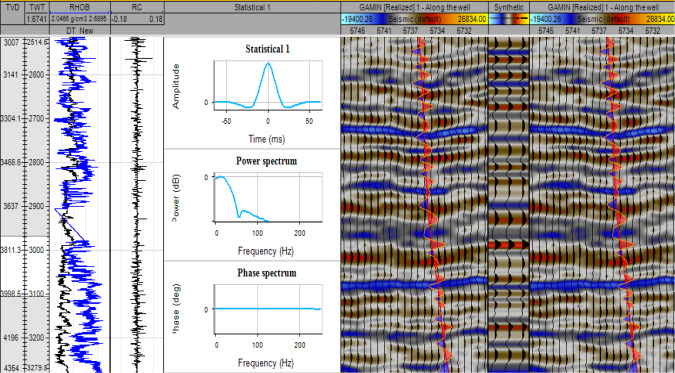
2. Generating Synthetic Seismogram:
– Acoustic Impedance Calculation: Using the sonic and density logs, acoustic impedance is calculated for the well. Acoustic impedance is the product of rock density and seismic velocity, and variations in impedance generate reflections.
– Reflectivity Series: The reflectivity series is derived from changes in acoustic impedance. It represents the theoretical reflection coefficients at each interface in the well.
– Wavelet Extraction: A seismic wavelet, representing the seismic source signature, is extracted from the seismic data. This wavelet is crucial for convolving with the reflectivity series to create the synthetic seismogram.
– Synthetic Seismogram Creation: The synthetic seismogram is generated by convolving the reflectivity series with the seismic wavelet. This synthetic seismogram represents the seismic response that would be recorded at the well location.

3. Correlation and Adjustment:
– Initial Correlation: The synthetic seismogram is initially compared with the actual seismic trace at the well location. The goal is to match key seismic events (peaks and troughs) between the synthetic and the seismic trace.
– Time-Depth Adjustment: Discrepancies between the synthetic and seismic data are addressed by adjusting the time-depth relationship. This may involve stretching or squeezing the synthetic seismogram to better match the seismic data.
– Wavelet Tuning: Further adjustments may be made to the wavelet to improve the match. This can include modifying the wavelet’s phase, amplitude, or frequency content to better align with the seismic data.

4. Finalizing the Tie:
– Cross-Correlation: The correlation between the synthetic seismogram and the seismic trace is quantified, typically using a cross-correlation coefficient. A high correlation indicates a good tie.
– Interpretation Validation: The final tie is validated by ensuring that the seismic events consistently match the geological and petrophysical information from the well across the section or volume.
– Application to Seismic Data: Once the tie is established, it can be applied to the entire seismic dataset, allowing for consistent interpretation across the survey area.

Challenges in Seismic to Well Ties

1. Wavelet Estimation:
– Variable Wavelet: The seismic wavelet can vary across the seismic section due to changes in acquisition parameters, processing, and subsurface conditions. Accurate wavelet estimation is critical but can be challenging.
– Phase and Frequency Issues: If the seismic data and the synthetic seismogram have different phases or frequency content, achieving a good tie can be difficult.

2. Data Quality:
– Seismic Data Quality: Poor seismic data quality, including issues like noise, multiples, or poor resolution, can complicate the seismic to well tie process.
– Log Data Quality: Inaccuracies or gaps in well log data, particularly the sonic log, can lead to errors in the synthetic seismogram and thus in the tie.

3. Velocity Model Accuracy:
– Velocity Variations: Accurate depth conversion relies on a correct velocity model. Velocity variations due to lithology changes, anisotropy, or fluid content can lead to mismatches between the seismic and well data.
– Checkshot and VSP Limitations: The accuracy of checkshot and VSP data is crucial for creating a reliable time-depth relationship. Errors or limitations in this data can affect the quality of the tie.

4. Complex Geology:
– Structural Complexity: In areas with complex geology, such as folding, faulting, or salt bodies, the seismic to well tie process becomes more difficult due to the complex wave propagation paths.
– Lateral Heterogeneity: Variations in lithology or fluid content away from the wellbore can cause discrepancies between the synthetic seismogram and the seismic data.

Applications of Seismic to Well Ties

1. Exploration and Prospecting:
– Prospect Evaluation: Seismic to well ties help in accurately evaluating exploration prospects by ensuring that seismic interpretations are grounded in well data.
– Identifying Direct Hydrocarbon Indicators (DHIs): A well-tied seismic section can help identify DHIs, such as bright spots or flat spots, which are indicative of hydrocarbon presence.

2. Reservoir Characterization:
– Lithology and Fluid Prediction: By accurately tying seismic data to well logs, geoscientists can better predict lithology and fluid content away from the well.
– Seismic Inversion: The process is critical for seismic inversion, where seismic data is converted into rock properties such as impedance, porosity, and saturation.

3. Well Planning:
– Drilling Decisions: Accurate seismic to well ties ensure that the depths of target formations are correctly predicted, aiding in well planning and reducing the risk of drilling failures.
– Geosteering: In horizontal or directional drilling, seismic to well ties provide the necessary data to steer the wellbore accurately within the reservoir.

4. 4D Seismic Monitoring:
– Time-Lapse Studies: In time-lapse (4D) seismic studies, where changes in the reservoir over time are monitored, seismic to well ties ensure that these changes are accurately interpreted in terms of reservoir performance and fluid movement.

Conclusion

Seismic to well ties are a foundational step in the integration of seismic data with well data, providing the necessary link between time-domain seismic reflections and depth-domain geological formations. This process enhances the accuracy of seismic interpretations, improves reservoir characterization, and aids in well planning and drilling. Despite challenges related to wavelet estimation, data quality, velocity model accuracy, and complex geology, seismic to well ties remain a critical tool in the exploration and production of hydrocarbons, ensuring that seismic data is reliably correlated with the subsurface reality as measured in wells.

Shallow hazard geophysical interpretation is a critical aspect of subsurface exploration and drilling operations, particularly in offshore environments. Shallow hazards are potential geologic or geophysical features near the seabed or the surface that pose risks to drilling and construction activities. These hazards include features like shallow gas, faults, overpressured zones, hard layers, and buried channels.

Importance of Shallow Hazard Interpretation

1. Safety in Drilling Operations:
– Identifying and understanding shallow hazards is crucial for the safe planning and execution of drilling operations. Hazards such as shallow gas can lead to blowouts if encountered unexpectedly during drilling.
– By predicting the presence of hazardous features, operators can design appropriate mitigation measures, such as adjusting drilling mud weights or rerouting well paths.

2. Cost Management:
– Encountering hazards during drilling can lead to significant delays, equipment damage, or even the abandonment of a well. Proper hazard identification helps avoid such costly incidents.
– Early identification of hazards allows for better planning and resource allocation, reducing the overall cost of drilling operations.

3. Environmental Protection:
– Shallow gas or hydrocarbons can pose environmental risks if accidentally released during drilling. Identifying these hazards beforehand enables operators to implement measures to prevent leaks or spills.
– Proper hazard interpretation helps minimize the risk of environmental contamination, protecting marine ecosystems and complying with regulatory requirements.

4. Infrastructure Stability:
– In addition to drilling, shallow hazard interpretation is essential for the stability of offshore platforms, pipelines, and other seabed infrastructure. Hazards like faulting or weak sediments can compromise the integrity of these structures.
– Identifying and mitigating these hazards ensures the long-term stability and safety of offshore infrastructure.

Types of Shallow Hazards

1. Shallow Gas:
– Definition: Shallow gas refers to gas accumulations at shallow depths, often within a few hundred meters of the seabed. These accumulations can be under pressure and are usually found in unconsolidated sediments.
– Risks: Encountering shallow gas during drilling can lead to gas kicks, blowouts, and loss of well control. It poses a significant safety risk to drilling operations.

2. Shallow Water Flows:
– Definition: These are water flows encountered at shallow depths, typically in deepwater environments. They occur in high-porosity, high-permeability sands and can cause significant operational challenges.
– Risks: Shallow water flows can erode the wellbore, destabilize the formation, and lead to well control issues.

3. Faults and Fractures:
– Definition: Faults and fractures near the surface can be associated with zones of weakness, increased permeability, or pathways for fluid migration.
– Risks: Drilling through faults or fractures can lead to loss of circulation, wellbore instability, and unexpected fluid encounters.

4. Overpressured Zones:
– Definition: Overpressured zones are areas where the pore pressure exceeds the normal hydrostatic pressure for a given depth. These zones can occur due to rapid sedimentation, fluid migration, or other geological processes.
– Risks: Encountering overpressured zones unexpectedly can result in well control issues, blowouts, or formation fracturing.

5. Buried Channels and Submarine Canyons:
– Definition: Buried channels and submarine canyons are ancient riverbeds or valleys that have been infilled with sediments. They often contain heterogeneous deposits, including sands, clays, and gravels.
– Risks: These features can lead to variable drilling conditions, including hard formations, fluid loss, and wellbore instability.

6. Hard Layers and Carbonate Hardgrounds:
– Definition: Hard layers, such as carbonate hardgrounds, are cemented or lithified layers near the seabed. They can pose challenges to drilling due to their hardness and abrasiveness.
– Risks: Drilling through hard layers can cause equipment damage, slow drilling rates, and difficulty in maintaining wellbore stability.

Geophysical Methods for Shallow Hazard Interpretation

1. Seismic Reflection Surveys:
– High-Resolution Seismic (HRS): HRS surveys are used to image shallow subsurface features with high detail. These surveys provide detailed images of stratigraphy, faults, and other potential hazards.
– 2D and 3D Seismic: Conventional 2D and 3D seismic surveys, although primarily used for deeper targets, can also be interpreted for shallow hazards. Attributes such as amplitude anomalies, flat spots, and bright spots may indicate shallow gas or fluid accumulations.

2. Seismic Attributes Analysis:
– Amplitude Analysis: High-amplitude reflections near the surface may indicate the presence of shallow gas or other fluid accumulations. Amplitude versus offset (AVO) analysis can further distinguish between gas and other lithologies.
– Seismic Inversion: Seismic inversion techniques can be used to convert seismic reflection data into impedance profiles, helping to identify lithological contrasts and potential hazards.

3. Seismic Velocity Analysis:
– Velocity Modeling: Anomalously low seismic velocities in shallow layers may indicate the presence of gas-charged sediments. Velocity analysis helps in identifying overpressured zones and weak formations.
– Velocity Pull-Up/Push-Down: Velocity anomalies can cause apparent structural highs (pull-up) or lows (push-down) in seismic data, which may indicate shallow hazards like gas pockets.

4. Seismic Refraction Surveys:
– Shallow Refraction: Seismic refraction surveys are useful for identifying hard layers, buried channels, and other features based on their velocity contrasts. This method is often used in conjunction with reflection surveys for a comprehensive shallow hazard assessment.

5. Electromagnetic Methods:
– Controlled-Source Electromagnetics (CSEM): CSEM surveys can detect resistive anomalies, which may indicate the presence of hydrocarbons or gas hydrates in shallow sediments.
– Marine Magnetotellurics (MT): MT methods are used to map resistivity variations in the subsurface, helping to identify gas hydrates, fluid accumulations, and other hazards.

6. Shallow Gas Indicators (SGIs):
– Direct Hydrocarbon Indicators (DHIs): Features like bright spots, flat spots, and gas chimneys observed in seismic data are common indicators of shallow gas.
– Seismic Chimneys: Vertical zones of disrupted seismic reflections, known as seismic chimneys, may indicate pathways for gas migration from deeper reservoirs to shallow depths.

Workflow for Shallow Hazard Interpretation

1. Data Collection and Preprocessing:
– Seismic Acquisition: High-resolution seismic data is acquired, ensuring sufficient coverage of the area of interest.
– Data Conditioning: The seismic data undergoes preprocessing, including noise attenuation, deconvolution, and multiple suppression, to enhance the quality of the shallow subsurface image.

2. Seismic Interpretation:
– Structural Interpretation: Identify and map faults, fractures, and other structural features that could pose hazards.
– Stratigraphic Interpretation: Interpret the shallow stratigraphy to identify potential sand bodies, channels, or other features associated with hazards.
– Attribute Analysis: Apply seismic attributes to highlight anomalies indicative of gas, overpressure, or other hazards.

3. Hazard Mapping and Risk Assessment:
– Hazard Identification: Based on seismic interpretation and attribute analysis, identify and map potential shallow hazards.
– Risk Assessment: Evaluate the likelihood and potential impact of each identified hazard, considering factors such as proximity to planned well paths or infrastructure.

4. Integration with Other Data:
– Well Data Integration: Integrate seismic interpretation with available well data, including shallow cores, logging while drilling (LWD), and mud logs, to validate and refine hazard interpretations.
– Geotechnical Data: Incorporate geotechnical survey data, such as cone penetration tests (CPT) or borehole data, to assess soil conditions and confirm the presence of hard layers or weak formations.

5. Mitigation Planning:
– Drilling Plan Adjustment: Modify drilling plans to avoid or mitigate identified hazards, such as rerouting well paths or adjusting drilling parameters.
– Monitoring and Contingency Planning: Implement real-time monitoring during drilling and develop contingency plans to respond to potential hazard encounters.

Challenges in Shallow Hazard Interpretation

1. Data Quality and Resolution:
– High-resolution data is essential for accurate shallow hazard interpretation, but acquiring and processing such data can be challenging, particularly in deepwater or complex environments.
– Noise, multiples, and other data quality issues can obscure shallow features, making interpretation difficult.

2. Complex Geology:
– Complex shallow geology, such as areas with numerous faults, channels, or varying lithologies, can complicate hazard identification and increase the risk of misinterpretation.
– Geological heterogeneity near the surface can lead to variable seismic responses, making it challenging to distinguish between different types of hazards.

3. Uncertainty in Interpretation:
– Shallow hazard interpretation often involves a degree of uncertainty, particularly when distinguishing between different potential causes of seismic anomalies, such as gas, water, or lithological changes.
– The non-uniqueness of geophysical data can lead to multiple plausible interpretations, requiring careful validation and integration with other data sources.

4. Environmental and Operational Constraints:
– Environmental factors, such as sea state, seabed conditions, and water depth, can impact data acquisition and the ability to accurately interpret shallow hazards.
– Operational constraints, such as time and budget limitations, may restrict the extent of shallow hazard assessment and the implementation of mitigation measures.

Conclusion

Shallow hazard geophysical interpretation is an essential component of offshore drilling and development projects,

Gravity and magnetic interpretation is a crucial aspect of geophysical exploration, particularly in the search for subsurface features and resources such as minerals, hydrocarbons, and geothermal reservoirs. These methods involve analyzing variations in the Earth’s gravitational and magnetic fields to infer the distribution of different rock types and geological structures beneath the surface.

Importance of Gravity and Magnetic Interpretation

1. Resource Exploration:
– Mineral Exploration: Gravity and magnetic surveys are widely used in the search for mineral deposits, such as iron ore, copper, and nickel. Magnetic data can reveal the presence of ferromagnetic minerals, while gravity data can detect denser rock bodies that may host valuable minerals.
– Hydrocarbon Exploration: In oil and gas exploration, these methods help in mapping subsurface structures like salt domes, fault systems, and basin geometry, which can serve as traps for hydrocarbons.
– Geothermal Exploration: Gravity and magnetic data are also used to identify favorable geological conditions for geothermal energy, such as faults, fractures, and volcanic structures.

2. Structural Mapping:
– Fault Detection: Gravity and magnetic surveys are effective in identifying and mapping faults, which are critical for understanding the structural framework of a region. This information is crucial for seismic hazard assessment and understanding fluid migration pathways.
– Basement Mapping: These methods help map the depth and shape of the crystalline basement, which is often important for understanding basin evolution, sediment distribution, and tectonic history.

3. Geotechnical and Environmental Applications:
– Engineering Projects: Gravity and magnetic surveys are used in site investigations for large engineering projects, such as tunnels, dams, and foundations, to detect subsurface anomalies that could affect stability.
– Environmental Studies: These methods can detect buried waste, cavities, or other subsurface features that may pose environmental hazards.

Gravity Interpretation

Fundamentals of Gravity Data

– Gravity Anomalies: Gravity surveys measure variations in the Earth’s gravitational field caused by differences in the density of subsurface materials. Positive anomalies typically indicate denser rocks (e.g., mafic intrusions), while negative anomalies suggest less dense materials (e.g., sedimentary basins).

– Bouguer and Free-Air Corrections: These corrections are applied to raw gravity data to account for the effects of elevation and topography, providing a more accurate representation of subsurface density variations.

Interpretation Techniques

1. Qualitative Interpretation:
– Anomaly Identification: Interpreters identify and map gravity anomalies, focusing on their shape, amplitude, and spatial distribution. These anomalies can indicate the presence of geological structures such as faults, folds, or intrusive bodies.
– Pattern Recognition: The spatial patterns of anomalies can help in distinguishing between different types of geological features, such as basins, ridges, or volcanic edifices.

2. Quantitative Interpretation:
– Gravity Modeling: Quantitative interpretation involves creating models of subsurface density distribution that explain the observed gravity anomalies. These models can be 2D or 3D, depending on the complexity of the geological setting.
– Inversion Techniques: Gravity inversion is a mathematical approach that converts gravity data into a 3D density distribution model. This method is used to estimate the depth, shape, and size of subsurface structures.

3. Depth Estimation:
– Euler Deconvolution: This technique helps estimate the depth to the source of gravity anomalies by analyzing the spatial gradient of the gravity field. It is widely used for quick depth estimates of faults, contacts, and other structures.
– Spectral Analysis: By analyzing the frequency content of gravity data, interpreters can estimate the depth of buried sources. This method is often used in regional studies to determine the thickness of sedimentary basins.

Magnetic Interpretation

Fundamentals of Magnetic Data

– Magnetic Anomalies: Magnetic surveys measure variations in the Earth’s magnetic field caused by the magnetization of subsurface rocks. Magnetic anomalies arise from the presence of ferromagnetic minerals, such as magnetite, within the Earth’s crust.

– Total Field and Residual Anomalies: The total magnetic field includes contributions from both regional (e.g., Earth’s main magnetic field) and local sources. Residual anomalies, which are often more relevant for geological interpretation, are obtained by subtracting the regional field.

Interpretation Techniques

1. Qualitative Interpretation:
– Magnetic Anomaly Mapping: Like gravity data, magnetic anomalies are mapped and analyzed for their amplitude, shape, and distribution. These maps help in identifying the location and extent of magnetic sources, such as igneous intrusions or mineral deposits.
– Magnetic Lineaments: Linear magnetic features can indicate the presence of faults, fractures, or lithological contacts. These lineaments are important for structural mapping and resource exploration.

2. Quantitative Interpretation:
– Magnetic Modeling: Magnetic data is modeled to estimate the depth, size, and magnetization of subsurface bodies. These models can be used to interpret the geology of an area and to identify potential resource targets.
– Magnetic Inversion: Similar to gravity inversion, magnetic inversion converts magnetic anomaly data into a 3D model of the subsurface magnetization distribution. This method helps in delineating the shape and depth of magnetic sources.

3. Depth Estimation:
– Depth to Magnetic Source: Techniques like Euler deconvolution, analytical signal, and tilt derivative are commonly used to estimate the depth to magnetic sources. These methods are valuable for identifying the depth of basement rocks, intrusions, and other geological features.
– Spectral Analysis: As with gravity data, spectral analysis of magnetic data can provide estimates of the depth to magnetic sources, particularly useful in regional studies.

Integrated Gravity and Magnetic Interpretation

1. Joint Interpretation:
– *omplementary Data: Gravity and magnetic data are often interpreted together because they provide complementary information. For example, gravity data is sensitive to density variations, while magnetic data is sensitive to variations in magnetization. Together, they offer a more complete picture of subsurface geology.
– Enhanced Structural Mapping: Integrating gravity and magnetic data can improve the accuracy of structural maps, particularly in areas with complex geology. This integration helps in correlating anomalies with geological features, such as faults, folds, and intrusions.

2. Case Studies in Exploration:
– Mineral Exploration: In mineral exploration, joint gravity and magnetic interpretation are used to identify targets such as massive sulfide deposits, which often have both a magnetic and a gravity signature due to their dense, magnetic mineral content.
– Hydrocarbon Exploration: Gravity and magnetic data are used together to map basin structures, identify salt domes, and delineate basement features, all of which are important for hydrocarbon exploration.

3. Software and Tools:
– Geophysical Software: Advanced software tools, such as Oasis montaj, Geosoft, and Petrel, are used for processing, modeling, and interpreting gravity and magnetic data. These tools allow for the integration of data from multiple sources and the creation of detailed subsurface models.
– 3D Visualization: Modern interpretation workflows often include 3D visualization, which helps geoscientists better understand the spatial relationships between different geological features and assess exploration risks and opportunities.

Challenges in Gravity and Magnetic Interpretation

1. Non-Uniqueness of Solutions:
– Interpretation Ambiguity: Gravity and magnetic data can sometimes lead to non-unique solutions, meaning that different subsurface models can explain the same data. This ambiguity requires careful validation and the integration of additional data, such as seismic or well data, to constrain interpretations.

2. Data Quality and Resolution:
– Survey Design: The quality and resolution of gravity and magnetic data depend on the survey design, including station spacing, altitude (for airborne surveys), and data acquisition parameters. Poor data quality can limit the ability to detect and interpret subtle anomalies.
– Noise and Artifacts: Noise and artifacts in the data, such as cultural noise (e.g., from infrastructure) or variations in the Earth’s main magnetic field, can complicate the interpretation process.

3. Complex Geology:
– Heterogeneous Terrains: In areas with complex geology, such as regions with multiple lithological units, fault systems, or volcanic activity, interpreting gravity and magnetic data can be challenging. These settings may require more sophisticated modeling and inversion techniques to achieve accurate results.

4. Depth Penetration Limits:
– Shallow vs. Deep Sources: Gravity and magnetic methods have different sensitivities to depth. While gravity data can provide information on deeper structures, magnetic data is often more sensitive to shallow sources. Balancing these sensitivities is important in integrated interpretations.

Conclusion

Gravity and magnetic interpretation plays a vital role in geophysical exploration, providing valuable insights into subsurface structures and resource potential. By analyzing variations in the Earth’s gravitational and magnetic fields, geoscientists can identify geological features, map structural frameworks, and target areas for further exploration. Despite challenges such as data quality, non-uniqueness of solutions, and complex geology, the integration of gravity and magnetic data, along with advanced modeling techniques, allows for robust and detailed interpretations that are critical for successful exploration and development projects.